
如何在 Jupyter 中使用 GeoPandas、cartopy 与 Natural Earth 可视化国家轮廓
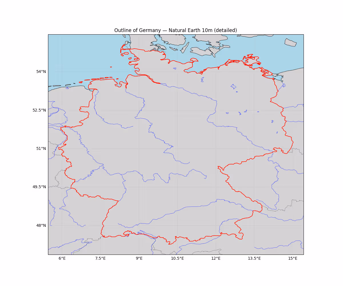
这个简单示例展示了如何在 Jupyter 中可视化一个国家的轮廓。本例中,我们将展示德国的轮廓。 为了使其在视觉上更具吸引力,我们还在背景中添加了其他国家的轮廓以及海洋。
我们使用 Natural Earth 10m 数据集,它会在此处自动下载。更大比例的变体(例如 1:110M)在此比例下无法提供足够的分辨率,视觉效果不佳。
VisualizeCountry.py
# 导入所需的库
import cartopy.crs as ccrs
import cartopy.feature as cf
from cartopy.feature import ShapelyFeature
import cartopy.io.shapereader as shpreader
import matplotlib.pyplot as plt
import geopandas as gpd
from shapely.ops import unary_union

# 使用 Plate Carree 投影创建地图
proj = ccrs.PlateCarree()
ax = plt.axes(projection=proj)
# 我们将拉取更高分辨率的 Natural Earth(10m)(如果可用)
# 使用 10m 的 'admin_0_countries' 以及海岸线/湖泊/河流以获取细节
try:
    # 读取 10m Natural Earth 国家数据,并通过 geopandas 提取德国几何图形以获得更好的精度
    countries = gpd.read_file(shpreader.natural_earth(resolution='10m', category='cultural', name='admin_0_countries'))
    germany = countries[countries['ISO_A3'] == 'DEU'].iloc[0].geometry
    # 用 0 缓冲修复任何无效的几何图形
    germany = germany.buffer(0)
    # 从几何图形确定一个紧凑的范围,并以度为单位添加少量边距
    minx, miny, maxx, maxy = germany.bounds
    pad_deg = 0.4
    extent = [minx - pad_deg, maxx + pad_deg, miny - pad_deg, maxy + pad_deg]
    ax.set_extent(extent, crs=ccrs.PlateCarree())

    # 添加高分辨率海岸线、边界以及湖泊/河流
    # 注意:这些都是可选的 - 只需注释掉你不需要的部分
    ax.add_feature(cf.LAND.with_scale('10m'), facecolor='lightgray')
    ax.add_feature(cf.OCEAN.with_scale('10m'), facecolor='lightblue')
    ax.add_feature(cf.COASTLINE.with_scale('10m'), lw=0.6)
    ax.add_feature(cf.BORDERS.with_scale('10m'), linestyle=':', lw=0.6)
    ax.add_feature(cf.LAKES.with_scale('10m'), facecolor='none', edgecolor='blue', lw=0.4)
    ax.add_feature(cf.RIVERS.with_scale('10m'), edgecolor='blue', lw=0.4)

    # 以更美观的样式添加德国多边形
    germany_feature = ShapelyFeature([germany], ccrs.PlateCarree(), facecolor='none', edgecolor='red', linewidth=1.2)
    ax.add_feature(germany_feature)

    # 添加网格线和标题
    gl = ax.gridlines(draw_labels=True, linestyle='--', linewidth=0.3)
    gl.top_labels = False
    gl.right_labels = False
    plt.gcf().set_size_inches(12, 10)
    ax.set_title('Outline of Germany — Natural Earth 10m (detailed)')

    plt.show()
except Exception as e:
    print(f"Error: {e}")
    print("Could not load 10m Natural Earth data. Falling back to built-in shapereader records with 110m resolution.")
    try:
        reader = shpreader.Reader(shpreader.natural_earth(resolution='110m', category='cultural', name='admin_0_countries'))
        germany = [c for c in reader.records() if c.attributes['NAME_LONG'] == 'Germany'][0]
        shape_feature = ShapelyFeature([germany.geometry], ccrs.PlateCarree(), facecolor='none', edgecolor='red', lw=2)
        ax.add_feature(cf.COASTLINE, lw=0.5)
        ax.add_feature(cf.BORDERS, linestyle=':', lw=0.5)
        ax.add_feature(shape_feature)
        plt.show()
    except Exception as e2:
print('Fallback also failed:', e2)Check out similar posts by category:
Geoinformatics
If this post helped you, please consider buying me a coffee or donating via PayPal to support research & publishing of new posts on TechOverflow