
How to compute Stokes drag in Python using UliEngineering
You can easily compute the drag force on a sphere moving through a viscous fluid using Stokes’ law with the UliEngineering Python library:
from UliEngineering.Physics.Viscosity import stokes_drag
from UliEngineering.EngineerIO import *

# Compute drag force on a 10 µm sphere in water
radius = 10e-6  # 10 µm
velocity = 0.01  # 1 cm/s
viscosity = 0.001  # Pa·s (water)

F = stokes_drag(radius, velocity, viscosity)
print(f"Drag force: {format_value(F, 'N')}")

# Compute drag force on a 1 µm sphere in water
radius = 1e-6
F = stokes_drag(radius, velocity, viscosity)
print(f"Drag force (1 µm sphere): {format_value(F, 'N')}")

# Compute drag force in more viscous fluid (glycerol)
viscosity = 1.412  # Pa·s (glycerol at 20°C)
F = stokes_drag(10e-6, velocity, viscosity)
print(f"Drag force in glycerol: {format_value(F, 'N')}")Example output
Drag force: 1.88 pN
Drag force (1 µm sphere): 188 fN
Drag force in glycerol: 2.66 nN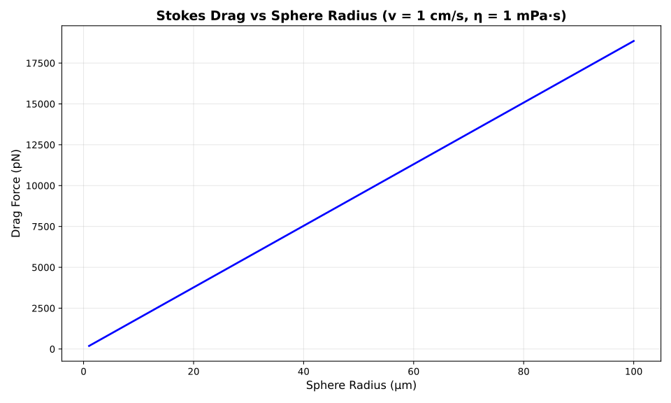
Stokes’ law is given by:
$$ F = 6 \pi \eta r v $$where $F$ is the drag force, $\eta$ is the dynamic viscosity, $r$ is the sphere radius, and $v$ is the velocity.
Stokes’ law describes the drag force on a sphere moving through a viscous fluid at low Reynolds numbers (typically Re < 1). This regime is called creeping flow or Stokes flow, where inertial effects are negligible compared to viscous effects. The linear relationship with velocity and radius makes this law particularly useful for analyzing small particles in fluids.
The plot above shows how the drag force varies with sphere radius for a fixed velocity of 1 cm/s in a water-like fluid (η = 1 mPa·s). Notice the linear increase in drag force with radius, as predicted by Stokes’ law.
This law is fundamental in many applications including sedimentation analysis, particle sizing, microfluidics, and understanding the motion of biological cells and nanoparticles in fluid environments.
Related posts
- How to compute Reynolds number in Python using UliEngineering
- How to compute kinematic viscosity in Python using UliEngineering
- How to compute Bingham stress in Python using UliEngineering
Plot generation script
#!/usr/bin/env python3
import matplotlib.pyplot as plt
import numpy as np
import sys
sys.path.insert(0, '/home/uli/dev/UliEngineering')

from UliEngineering.Physics.Viscosity import stokes_drag

# Sphere radius range for plotting
r = np.linspace(1e-6, 1e-4, 100)  # 1 µm to 100 µm

# Create plot
plt.figure(figsize=(10, 6))

# Fixed parameters
velocity = 0.01  # m/s
viscosity = 0.001  # Pa·s (water-like)

# Calculate drag force
F = stokes_drag(r, velocity, viscosity) * 1e12  # Convert to pN

plt.plot(r * 1e6, F, color='blue', linewidth=2)
plt.xlabel('Sphere Radius (µm)', fontsize=12)
plt.ylabel('Drag Force (pN)', fontsize=12)
plt.title('Stokes Drag vs Sphere Radius (v = 1 cm/s, η = 1 mPa·s)', fontsize=14, fontweight='bold')
plt.grid(True, alpha=0.3)

plt.tight_layout()
plt.savefig('stokes_drag_plot.svg', format='svg', dpi=300)
print("Plot saved to stokes_drag_plot.svg")