
How to compute Poiseuille flow rate in Python using UliEngineering
You can easily compute the volumetric flow rate for laminar flow in cylindrical pipes using Poiseuille’s law with the UliEngineering Python library:
from UliEngineering.Physics.Viscosity import poiseuille_flow_rate
from UliEngineering.EngineerIO import *

# Compute flow rate for a 5mm radius pipe
radius = 0.005  # 5mm in meters
pressure_drop = 1000.0  # Pa
length = 1.0  # m
viscosity = 0.001  # Pa·s (water)

Q = poiseuille_flow_rate(radius, pressure_drop, length, viscosity)
print(f"Flow rate: {format_value(Q, 'm³/s')}")

# Compute flow rate for a 10mm radius pipe
radius = 0.01
Q = poiseuille_flow_rate(radius, pressure_drop, length, viscosity)
print(f"Flow rate (10mm pipe): {format_value(Q, 'm³/s')}")

# Compute flow rate with higher pressure drop
pressure_drop = 5000.0
Q = poiseuille_flow_rate(0.005, pressure_drop, length, viscosity)
print(f"Flow rate (5kPa drop): {format_value(Q, 'm³/s')}")Example output
Flow rate: 4.91 mL/s
Flow rate (10mm pipe): 78.5 mL/s
Flow rate (5kPa drop): 24.5 mL/s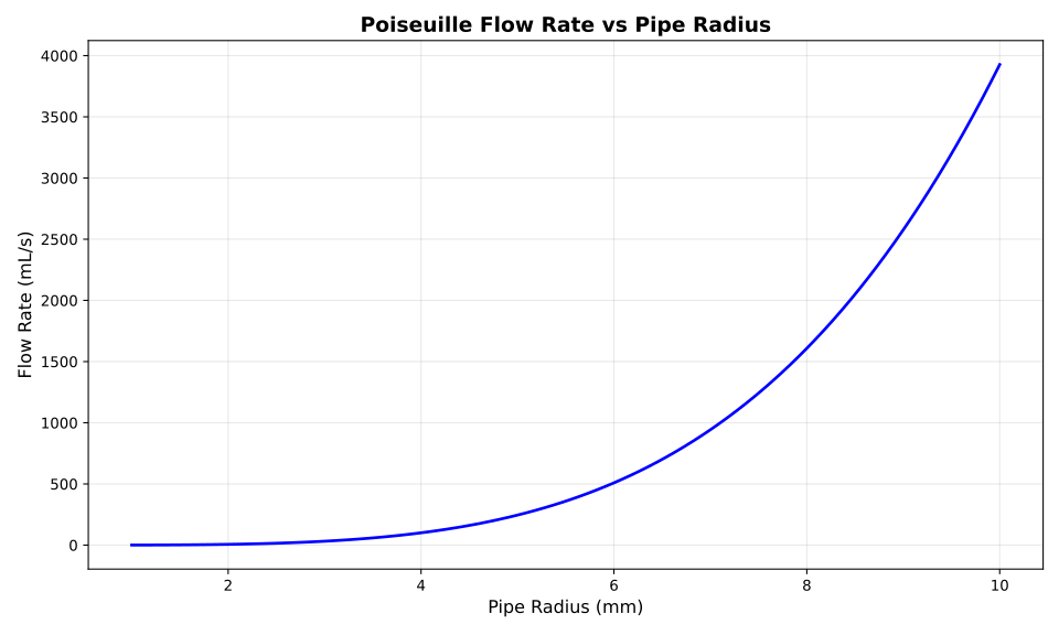
Poiseuille’s law is given by:
$$ Q = \frac{\pi \cdot r^4 \cdot \Delta P}{8 \cdot \eta \cdot L} $$where $Q$ is the volumetric flow rate, $r$ is the pipe radius, $\Delta P$ is the pressure drop along the pipe, $\eta$ is the dynamic viscosity, and $L$ is the pipe length.
Poiseuille’s law describes laminar flow in cylindrical pipes and is valid for Reynolds numbers below approximately 2300. The strong dependence on the fourth power of the radius means that doubling the pipe radius increases the flow rate by a factor of 16.
The plot above shows how the flow rate varies with pipe radius for a fixed pressure drop, length, and viscosity. Notice the dramatic increase in flow rate as the radius increases, following the $r^4$ relationship.
This law is fundamental to fluid dynamics and is used in applications ranging from blood flow analysis to pipeline design and microfluidics.
Related posts
- How to compute Bingham stress in Python using UliEngineering
- How to compute Reynolds number in Python using UliEngineering
- How to compute kinematic viscosity in Python using UliEngineering
Plot generation script
#!/usr/bin/env python3
import matplotlib.pyplot as plt
import numpy as np
import sys
sys.path.insert(0, '/home/uli/dev/UliEngineering')

from UliEngineering.Physics.Viscosity import poiseuille_flow_rate

# Pipe radius range for plotting
r = np.linspace(0.001, 0.01, 100)  # 1mm to 10mm

# Create plot
plt.figure(figsize=(10, 6))

# Fixed parameters
pressure_drop = 1000.0  # Pa
length = 1.0  # m
viscosity = 0.001  # Pa·s (water-like)

# Calculate flow rate
Q = poiseuille_flow_rate(r, pressure_drop, length, viscosity) * 1e6  # Convert to mL/s

plt.plot(r * 1000, Q, color='blue', linewidth=2)
plt.xlabel('Pipe Radius (mm)', fontsize=12)
plt.ylabel('Flow Rate (mL/s)', fontsize=12)
plt.title('Poiseuille Flow Rate vs Pipe Radius', fontsize=14, fontweight='bold')
plt.grid(True, alpha=0.3)

plt.tight_layout()
plt.savefig('poiseuille_plot.svg', format='svg', dpi=300)
print("Plot saved to poiseuille_plot.svg")