
How to compute Bingham plastic stress in Python using UliEngineering
You can easily compute the shear stress for Bingham plastic fluids using the UliEngineering Python library. The Bingham plastic model describes fluids that behave like solids at low shear stress and flow like liquids above a yield stress:
from UliEngineering.Physics.Viscosity import bingham_stress, BinghamConstants
from UliEngineering.EngineerIO import *

# Compute Bingham stress with default constants
gamma = 10.0  # Shear rate in s^-1
tau = bingham_stress(gamma)
print(f"Shear stress at {gamma} s^-1: {format_value(tau, 'Pa')}")

# Compute Bingham stress for drilling mud
drilling_mud = BinghamConstants(name='Drilling mud', tau0=20.0, mu_p=0.3)
gamma = 25.0
tau = bingham_stress(gamma, drilling_mud)
print(f"Drilling mud shear stress at {gamma} s^-1: {format_value(tau, 'Pa')}")

# Compute Bingham stress for toothpaste
toothpaste = BinghamConstants(name='Toothpaste', tau0=50.0, mu_p=0.5)
gamma = 5.0
tau = bingham_stress(gamma, toothpaste)
print(f"Toothpaste shear stress at {gamma} s^-1: {format_value(tau, 'Pa')}")Example output
Shear stress at 10.0 s^-1: 11.0 Pa
Drilling mud shear stress at 25.0 s^-1: 27.5 Pa
Toothpaste shear stress at 5.0 s^-1: 52.5 Pa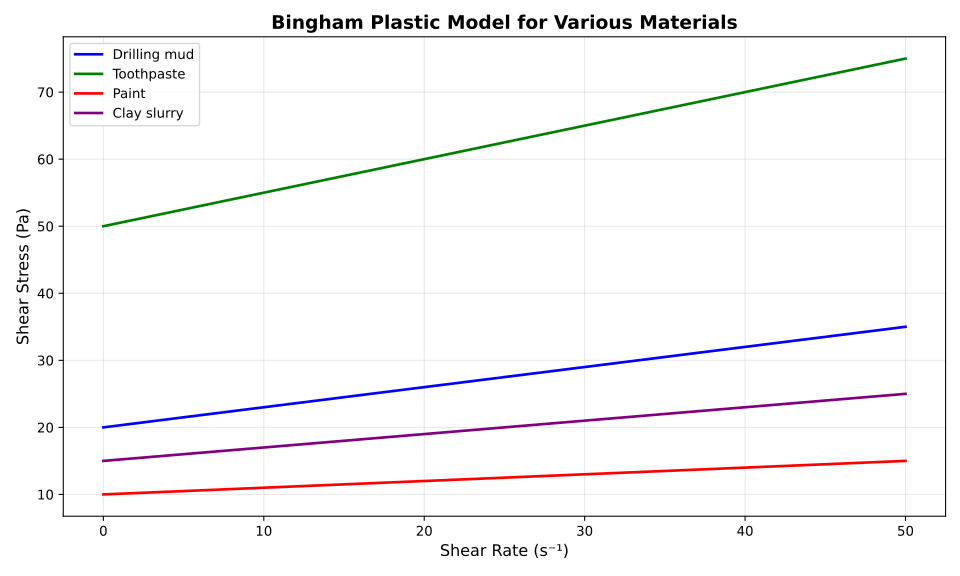
The Bingham plastic model is given by:
$$ \tau = \tau_0 + \mu_p \cdot \dot{\gamma} $$where $\tau$ is the shear stress, $\tau_0$ is the yield stress (minimum stress required to initiate flow), $\mu_p$ is the plastic viscosity, and $\dot{\gamma}$ is the shear rate.
Bingham plastics are non-Newtonian fluids that exhibit a yield stress below which they behave like solids. Above this yield stress, they flow with a constant plastic viscosity. Common examples include drilling muds, toothpaste, paints, and certain food products like ketchup.
The plot above shows the Bingham plastic model for various materials over a range of shear rates. Notice that all materials have a non-zero intercept (yield stress) and then increase linearly with shear rate, with the slope determined by the plastic viscosity.
The UliEngineering library provides the BinghamConstants dataclass for defining material-specific yield stress and plastic viscosity parameters. If no constants are provided, default example values (τ₀ = 10 Pa, μₚ = 0.1 Pa·s) are used.
Related posts
- How to compute Poiseuille flow rate in Python using UliEngineering
- How to compute Stokes drag in Python using UliEngineering
- How to compute Reynolds number in Python using UliEngineering
Plot generation script
#!/usr/bin/env python3
import matplotlib.pyplot as plt
import numpy as np
import sys
sys.path.insert(0, '/home/uli/dev/UliEngineering')

from UliEngineering.Physics.Viscosity import (
    bingham_stress,
    BinghamConstants,
)

# Shear rate range for plotting
gamma = np.linspace(0, 50, 100)  # 0 to 50 s^-1

# Create plot
plt.figure(figsize=(10, 6))

# Plot for different Bingham materials
materials = [
    ('Drilling mud', BinghamConstants(name='Drilling mud', tau0=20.0, mu_p=0.3), 'blue'),
    ('Toothpaste', BinghamConstants(name='Toothpaste', tau0=50.0, mu_p=0.5), 'green'),
    ('Paint', BinghamConstants(name='Paint', tau0=10.0, mu_p=0.1), 'red'),
    ('Clay slurry', BinghamConstants(name='Clay slurry', tau0=15.0, mu_p=0.2), 'purple'),
]

for name, constants, color in materials:
    tau = bingham_stress(gamma, constants)
    plt.plot(gamma, tau, label=name, color=color, linewidth=2)

plt.xlabel('Shear Rate (s⁻¹)', fontsize=12)
plt.ylabel('Shear Stress (Pa)', fontsize=12)
plt.title('Bingham Plastic Model for Various Materials', fontsize=14, fontweight='bold')
plt.legend(loc='upper left', fontsize=10)
plt.grid(True, alpha=0.3)

plt.tight_layout()
plt.savefig('bingham_plot.svg', format='svg', dpi=300)
print("Plot saved to bingham_plot.svg")